Wind Turbine Aerodynamics - 4a - Rotor Aerodynamics

15 August 2026, Galih Bangga

Kinematics of Blade Section

Wind turbine blade is usually long and slender - the spanwise flow << streamwise flow - 2D assumption is mostly valid, only at the root and tip, more complex flow has to be considered.

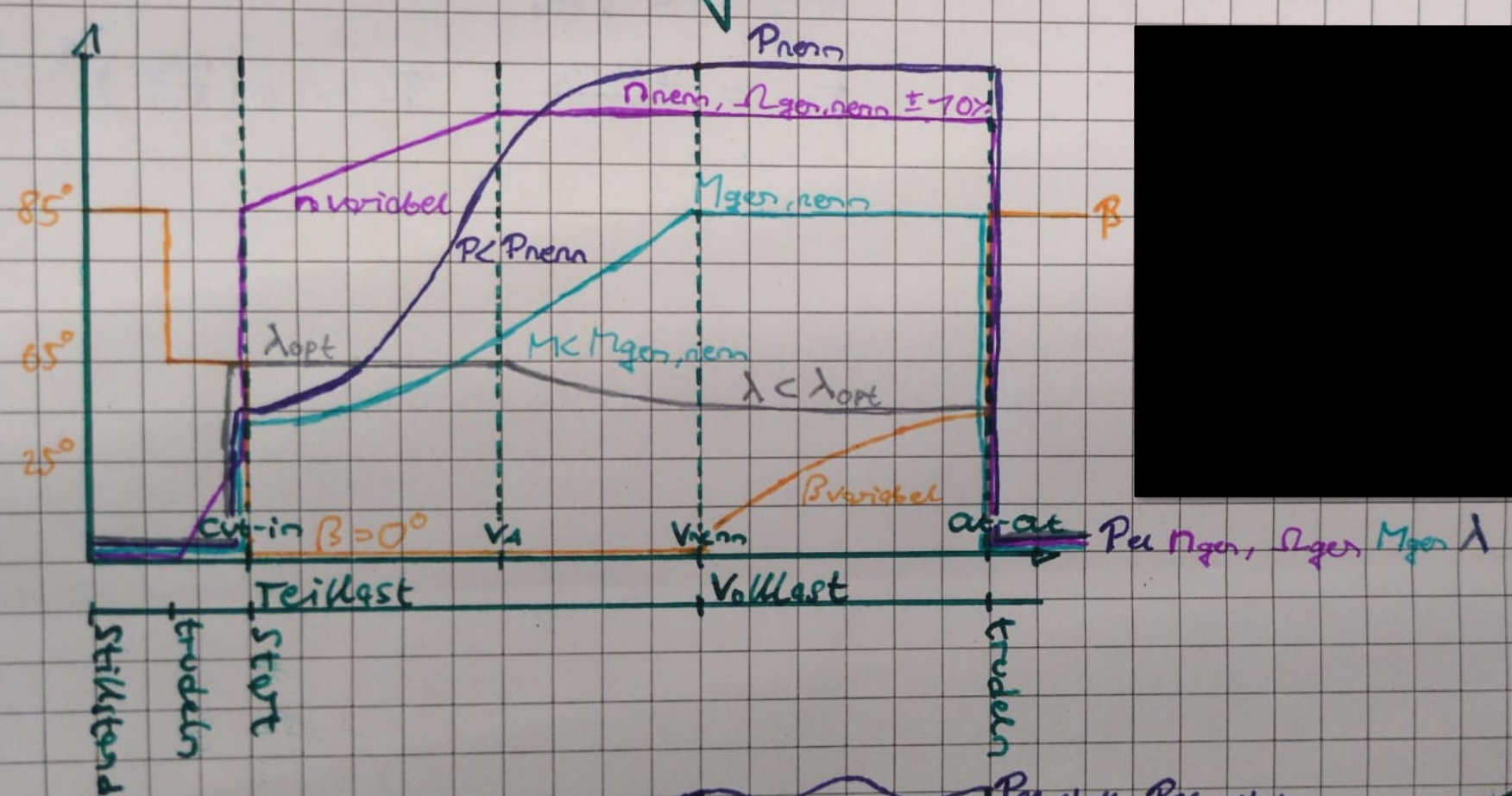
Rotor Operation Modes - Power production

Rated generator power is reached at $v_{nenn}$, while the rated generator power is reached at $v_{rated}. They are not necessarily the same.

Rotor Operation Modes - Stand-still

• Parked
  • Brakes applied, rotor rotation prevented
• Idling
  • Orienting the turbine blades or nacelle to brake aerodynamically
  • If possible, idling is better, because no break is needed, loads not as high

Dynamic Stall

• Massively separated flow which includes all complex characteristics
• Unsteady excitation from angle of attack variation
• Strong vertex interactions on blade airfoil surface
  • Leading edge vortex LEV
  • Trailing edge vortex TEV

$$ k = \frac{\pi \cdot f \cdot c}{U_{\infty}} $$

• $k$: Reduced frequency

• $k = 0$: steady state aerodynamics

• $0 < k < 0,05$: quasi steady aerodynamics

• $k > 0,05$: unsteady aerodynamics

• HAWT

  • turbulence
  • wind shear in the boundary layer of the ground
  • gusts lead to altering the angle of attack
  • yaw of the turbine
  • wind turbine in parked / idling

• VAWT

  • dynamic stall by design for low tip speed ratios
  • negative to positive angle of attack

How to model dynamic stall in engineering simulations:

This seems to be an important topic, lecturer Galih Bangga has written a paper on it!

• Indicial formulation
  • representing a response of the airfoil parameters such as the delayed unsteady angle of attack, separation point and unsteady force based on the unsteady excitation such as the rate-of-change of the angle of attack
  • no need for time integration, numerically stable
  • cannot be used for steady-state stability analysis of the turbine for controller design
• State-space representation
  • representing the dynamic conditions in th sets of differential equations, commonly first or second order ordinary differential equations ODEs
  • solution depends on time integrator being used, may be unstable if no proper integration method is used or if time step is too large
  • can be used for steady-state stability analysis of the turbine for controller design

Tip loss effects

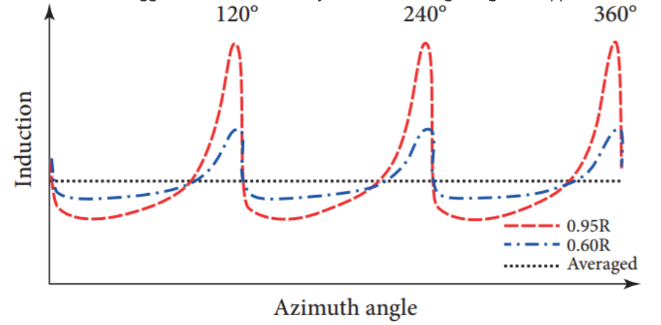
Can be seen as limitation of the momentum theory (see next lecture), which assumes a constand loading across the rotor plane. Can also be seen as the deviation of the 2D airfoil data and the 3D conditions

As the radial pressure gradient approaching the tip becomes stronger, the flow becomees more three dimensional - the actual angle of attack seen by the blade section becomes smaller due to the downwash effect Attained lift is smaller than in idealized conditions

• loading is not uniform across rotor plane
• maximum in blade locations
• variation becomes greater approaching the tip area

Himmelskamp Effects

Doctoral thesis of the lecturer, probably important to understand for the exam

Rotating blade - effect of centrifugal and coriolis force

• Centrifugal force pushes air towards the outer regions - creates radial component in the flow field
• Coriolis force is acting towards the trailing edge

Because of Himmelskamp effects, at large angles of attack, 3D simulations have higher lift and delayed stall compared to 2D simulations

• Stall delay -> infinity: only coriolis force in chordwise direction
• Stall delay -> zero: only centrifugal force in spanwise direction

Questions in the end

• What are the different characteristics between leading edge stall and trailing edge stall?
• what is the reduced frequency?
• what are the main steps in the dynamic stall formation?
• examples of dynamic stall models?
• what is the tip loss effect of a rotor?
• what causes the stall delay and lift enhancement?